Step-by-step tutorial for functions in deepszsim

This tutorial will explore the functions included in the deepszsim code from DeepSkies. For the overall simulation function description see demo_simulation.ipynb.

Imports

import deepszsim

import numpy as np
import matplotlib.pyplot as plt
import time
import h5py

from astropy.constants import M_sun, G, sigma_T, m_e, c, h, k_B
from astropy import units as u
from decimal import Decimal

Next, we make a dictionary from the variables input.yaml. We then load in the keys from the dictionary to create our variables.

d=deepszsim.load_vars() #Make a dictionary and cosmology from the .yaml
d.keys()

dict_keys(['survey', 'survey_freq', 'beam_size_arcmin', 'noise_level', 'image_size_pixels', 'pixel_size_arcmin', 'image_size_arcmin', 'cosmo', 'sigma8', 'ns'])

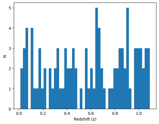
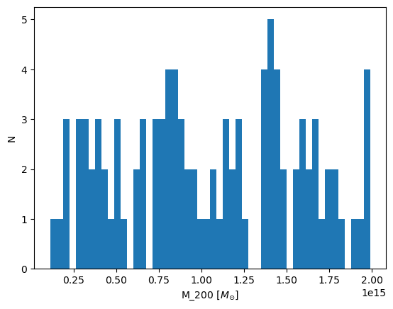
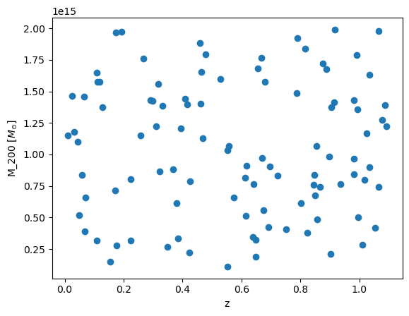
Next, we create a new flat redshift and mass (here, M_200, as defined relative to the critical density) distribution using the function flastdist_halo from dm_halo_dist which uses random uniform generation. Our distribution saved to a h5 file titled massdist.h5. Below are three graphs, showing the redshift distribution, mass distribution, and redshift and mass scatterplot.

#Generate a new flat z, M_200 distribution and save to file:
nsources = 100 #Number of halos to generate
zdist, mdist=deepszsim.dm_halo_dist.flatdist_halo(0.01,1.1,1e14,2e15,nsources) #Generate a flat z, M_200 distribution for sims

plt.hist(zdist,bins=50) #Show the z distribution
plt.ylabel('N'),plt.xlabel('Redshift (z)')
plt.show()
plt.hist(mdist,bins=50) #Show the M_200 distribution
plt.ylabel('N'),plt.xlabel(r'M_200 [$M_{\odot}$]')
plt.show()
plt.plot(zdist,mdist,'o') #Show the z, M_200 scatterplot
plt.xlabel('z'),plt.ylabel(r'M_200 [$M_{\odot}$]')
plt.show()

sourceid=int(time.time()) #Create an initial ctime for the halo ID list to save catalog
idlist=[sourceid+x for x in range(len(zdist))] #Create the halo ID list for catalog

#Save this array to a h5 file
data = h5py.File('massdist.h5', 'w')
data.create_dataset('Redshift', data=zdist)
data.create_dataset('Mass', data=mdist)
data.create_dataset('id', data=idlist)
data.close()

Now we are able to read our h5 file to access the distributions. We load the redshift distribution to the variable zdist, mass distribution to mdist and the list of ids corresponding to each halo to idlist.

with h5py.File('massdist.h5', 'r') as data:
    zdist = data['Redshift'][()]
    mdist = data['Mass'][()]
    idlist = data['id'][()]

Simulating SZ submaps using these halos

The following code walks through how to use methods in deepszsim in order to generate simulated SZ submaps.

The following values are examples for the purpose of the tutorial. We create a radius array of 1000 values, from 0.01 to 10 in units of arcmin. We then convert to Mpc. Next we initialize example redshift and \(M_{200}\) values. We then get \(R_{200}\) and \(c_{200}\) values from our \(M_{200}\) value from Colossus.

r=np.linspace(0.01, 10, 1000) #arcmin
r=deepszsim.utils.arcmin_to_Mpc(r,d["pixel_size_arcmin"],d["cosmo"])

z=0.5 #example redshift
M200=2e14 #example M_200 in solar masses

(M200,R200,_,c200)=deepszsim.make_sz_cluster.get_r200_angsize_and_c200(M200, z, load_vars_dict=d) #Use M200 to get R200 and concentration from Colossus

Thermal Pressure Profile Generation

This section will walk through how to generate thermal pressure profiles using equations from Battaglia 2012 Section 4 (The Thermal Pressure Profile).

\[P_\Delta = GM_\Delta\Delta\rho_{cr}(z)f_b/(2R_\Delta)\]

P200 represents the \(R_{200}\) normalized thermal pressure profile for a cluster of galaxies.

P200 = deepszsim.make_sz_cluster.P200_Battaglia2012(M200, z, R200_Mpc=R200, load_vars_dict=d) #P200 from Battaglia et al. 2012

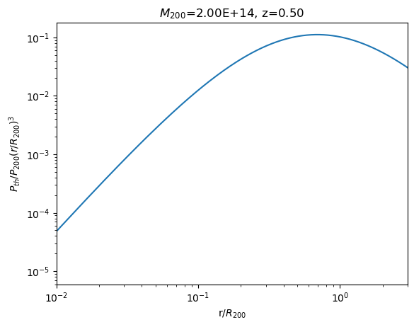
Here we generate fit parameters for a restricted version of a NFW profile. The input weights are chosen to be the inverse variances of fit parameter values from the individual pressure fits for each cluster within the bin.

• P0: amplitude

• xc: core-scale

• beta: power law index for the asymptotic fall off of the profile.

Pth, generated in the next block of code, is the restricted version of the NFW profile. We scale Pth by $ (r/R_{200})^3 $, like in Battaglia 2012.

P0 = deepszsim.make_sz_cluster._P0_Battaglia2012(M200,z) #Parameter computation from Table 1 Battaglia et al. 2012
xc = deepszsim.make_sz_cluster._xc_Battaglia2012(M200,z)
beta = deepszsim.make_sz_cluster._beta_Battaglia2012(M200,z)

Pth = deepszsim.make_sz_cluster.Pth_Battaglia2012(r, M200, z, d, R200_Mpc=R200) #Output Battaglia 2012 pressure profile

Pth_rescaled=(Pth)*(r/R200)**3.

Here, we graph the rescaled Pth on a log-log plot against \((r/R_{200})\).

plt.plot(r/R200,Pth_rescaled) #Plot Battaglia 2012 pressure profile
plt.xscale('log')
plt.yscale('log')
plt.ylabel('$P_{th}/P_{200}(r/R_{200})^3$')
plt.xlabel('r/$R_{200}$')
plt.title('$M_{200}$='+f'{M200:.2E}, z={z:0.2f}') #solar masses, redshift
plt.xlim(.010,3)
plt.show()

Compton-y Profile Generation

Next, utilizing our pressure profile Pth, we find the Compton-y parameter (y) by utilizing the line of sight integral:

\[Y_\Delta = \frac{\sigma_T}{m_e c^2} \int_0^{R_{200}} P_e(r)4\pi r^2 \, dr\]

y = deepszsim.make_sz_cluster.Pe_to_y(deepszsim.make_sz_cluster.Pth_Battaglia2012, r,
                                  M200, z, d, R200_Mpc=R200)

only implementing `Battaglia2012` for profile

y[0] #print central y value

2.4177567672074464e-05

Next, we find the corresponding temperatures from the central y value y[0]. We do this by utilizing the function f_sz which uses the equation:

\[\frac{\mathrm{dT}_{tsz} (\theta)}{\mathrm{T}_{CMB}} = f_{sz} y(\theta),\]

where \(y(\theta)\) is the Compton parameter at a projected angle \(\theta\) from the cluster center.

fSZ=deepszsim.simtools.f_sz(150,d["cosmo"].Tcmb0) #get f_SZ for observation frequency of 30 GHz
dT=d["cosmo"].Tcmb0*y[0]*fSZ #get dT from y0 using f_SZ
dT=dT.to(u.uK) #Convert to uK
print(dT)

-62.78590777743287 uK

This is the generated 1D Compton-y profile, which plots our Compton-y profile y against the radius in Mpc.

plt.plot(r, y)
plt.xlabel('Radius [Mpc]')
plt.ylabel('Compton-y')
plt.xscale('log')
plt.xlim(0.006,1)
plt.title('Compton-y Profile vs. Radius, $M_{200}$='+f'{M200:.2E}, z={z:0.2f}')
plt.show()

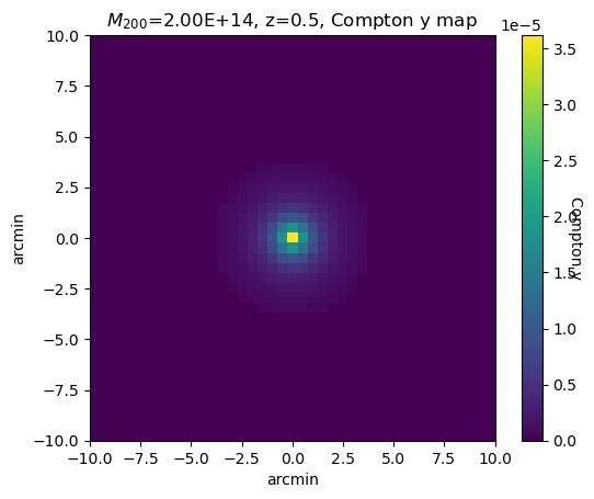
Profile Visualization

The end goal of this section is to generate a convolved CMB map + SZ cluster with noise.

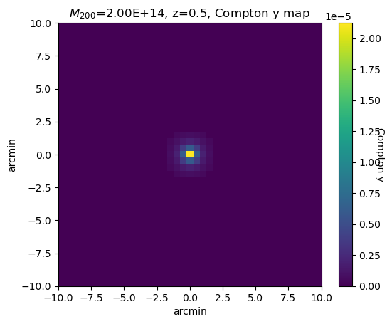
In order to create a Compton y map, we utilize the make_y_submap function. This 2D submap has different values than the y above, because of the different pixelization choices.

width = 10
y_map = deepszsim.make_sz_cluster.generate_y_submap(M200, z, load_vars_dict=d, R200_Mpc=R200)
deepszsim.visualization.plot_graphs(y_map,'$M_{200}$='+'{:.2E}'.format(Decimal(M200))+', z='+str(z)+', Compton y map',
                          'arcmin', 'arcmin', 'Compton y', width=10)
print(f'y_max = {y_map.max()}, y_min = {y_map.min()}')

y_max = 2.1240205860820517e-05, y_min = 0.0

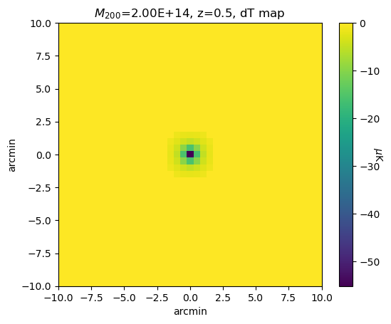
Next, we plot the temperature map, using the \(f_{sz}\) equation again:

\[\frac{\mathrm{dT}_{tsz} (\theta)}{\mathrm{T}_{CMB}} = f_{sz} y(\theta)\]

dT_map = (y_map * d["cosmo"].Tcmb0 * fSZ).to(u.uK).value
deepszsim.visualization.plot_graphs(dT_map, '$M_{200}$='+'{:.2E}'.format(Decimal(M200))+', z='+str(z)+', dT map',
                                'arcmin', 'arcmin', '$\mu$K', width=10)

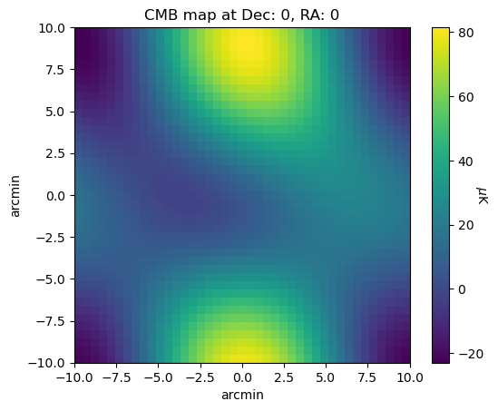
CMB submap generation

This is an example of what a generated CMB map will look like. We use the function get_cls in the simtools file to generate a power spectrum, which we then use to create the CMB map using make_cmb_map. This is just an example CMB map; it doesn’t carry forward to the cells below.

ps = deepszsim.simtools.get_cls(ns=d["ns"], cosmo=d["cosmo"])
cmb_map = deepszsim.simtools.make_cmb_map(shape=y_map.shape, pix_size_arcmin=d["pixel_size_arcmin"], ps=ps)*u.uK
deepszsim.visualization.plot_graphs(cmb_map.value,'CMB map at Dec: 0, RA: 0',
                                'arcmin','arcmin','$\mu$K', width=10)

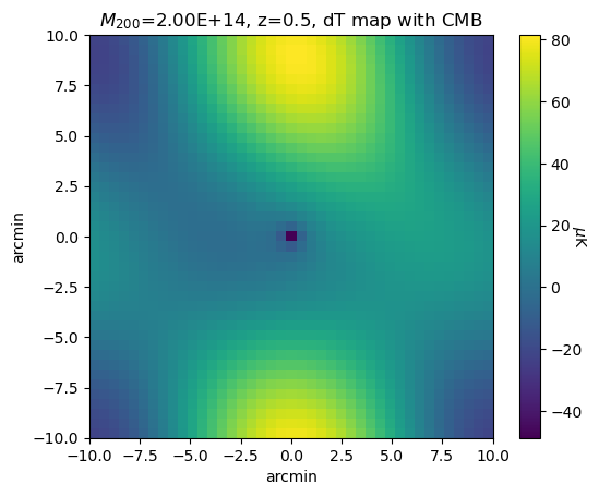
Creating a signal (SZ + CMB) map

This is an example of what a generated signal map will look like.

signal_map = dT_map + cmb_map.value
deepszsim.visualization.plot_graphs(signal_map,'$M_{200}$='+'{:.2E}'.format(Decimal(M200))+', z='+str(z)+', dT map with CMB',
                                'arcmin','arcmin','$\mu$K',width=10)

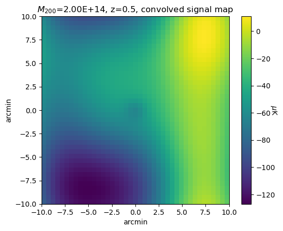
Beam Convolution

This what an example CMB map post beam-convolution will look like. Here we use the method add_cmb_map_and_convolve in simtools, which creates a CMB map, adds our cluster, convolves with a beam, and then eliminates edge effects.

conv_map, _ = deepszsim.simtools.add_cmb_map_and_convolve(dT_map, ps, d["pixel_size_arcmin"], d["beam_size_arcmin"])
deepszsim.visualization.plot_graphs(conv_map,'$M_{200}$='+'{:.2E}'.format(Decimal(M200))+', z='+str(z)+', convolved signal map',
                                'arcmin','arcmin','$\mu$K',width = 10)

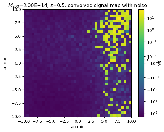
Adding Noise

Next, we add a white noise map to the convolved CMB map using the generate_noise_map function in noise.

noise_map=deepszsim.noise.generate_noise_map(d["image_size_pixels"], d["noise_level"], d["pixel_size_arcmin"])
total_map=conv_map + noise_map
deepszsim.visualization.plot_graphs(total_map,'$M_{200}$='+'{:.2E}'.format(Decimal(M200))+', z='+str(z)+', convolved signal map with noise',
                                'arcmin','arcmin','$\mu$K', width = 10, extend=True, logNorm = True)
print("noise level is " + str(d["noise_level"]) +  'uK*arcmin')

noise level is 8uK*arcmin

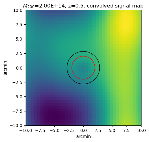
Aperture Photometry

We can use the function get_tSZ_signal_aperture_photometry from filters to associate an tSZ signal to our cluster. This is a demonstration of how to use the aperture photometry tool.

ap_arcmin=2.0 #arcminutes
pix_scale=0.5 #each pixel is 0.5 arcmin
disk, ring, signal = deepszsim.filters.get_tSZ_signal_aperture_photometry(conv_map, ap_arcmin, pix_scale)
print('Average in inner radius: '+str(disk))
print('Average in outer radius: '+str(ring))
print('tSZ signal: '+str(signal))
center = np.array(conv_map.shape) / 2
center = center - center[0]
fig, ax = plt.subplots()
ax.imshow(conv_map, extent=[-width,width,-width,width])
disk_circle = plt.Circle(center, ap_arcmin, color='red', fill=False, linewidth=1)
annulus_circle = plt.Circle(center, ap_arcmin * np.sqrt(2), color='black', fill=False, linewidth=1)
ax.add_patch(disk_circle)
ax.add_patch(annulus_circle)
plt.ylabel('arcmin')
plt.xlabel('arcmin')
plt.title('$M_{200}$='+'{:.2E}'.format(Decimal(M200))+', z='+str(z)+', convolved signal map')
plt.show()

Average in inner radius: -53.947394172732494
Average in outer radius: -49.42236198587485
tSZ signal: -4.5250321868576435

Creating Sims without step by step functions

For more on overall sim generating functions see demo_simulation.ipynb.

If you want to create simulated clusters without previously defining a mass and redshift distribution, you can use the simulate_clusters class in make_sz_cluster.py. You can specify the following characteristics of the simulated clusters:

• \(M_{200}\)

• redshift

• number of halos

• halo parameters

• \(R_{200}\)

We will create a galaxy cluster of 10 halos as an example:

cl = deepszsim.simclusters.simulate_clusters(num_halos=10)

making 10 clusters uniformly sampled from0.1<z<1.1, and 4.0e+13<M200<1.0e+15

The simulate_clusters class has multiple methods to get different characteristics of the simulated clusters.

• Compton-y map: get_y_map

• dT map: get_dT_map

• Temperature map: get_T_map

• ith map of the sky: get_ith_map

simulated_map = cl.get_y_maps()[0]
deepszsim.visualization.plot_graphs(simulated_map,'$M_{200}$='+'{:.2E}'.format(Decimal(M200))+', z='+str(z)+', Compton y map',
                                'arcmin','arcmin','Compton y',width=10, extend=True)

_ = cl.get_T_maps()

k = list(cl.clusters.keys())
k

['0347177_028_078954',
 '0163978_055_250734',
 '0900430_044_200930',
 '0611437_042_462385',
 '0928287_020_156564',
 '0845614_026_237929',
 '0624573_108_676349',
 '0097185_062_847315',
 '0272504_089_925013',
 '0628552_094_549938']

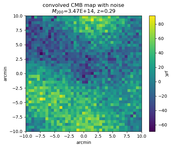
We can extract specific maps from specific simulated clusters. For example, the code below visualizes the final_map (beam convolved temperature map + CMB + noise) for the first simulated cluster (index 0). (To be able to access the maps, you must run cl.get_T_maps() first!)

cluster_ex0 = cl.clusters[k[0]]
simulated_map = cluster_ex0['maps']['final_map']
deepszsim.visualization.plot_graphs(simulated_map,
                                    "convolved CMB map with noise\n"+\
                                    '$M_{200}$='+f"{cluster_ex0['params']['M200']:.2E}, z={cluster_ex0['params']['redshift_z']:.2}",
                                    'arcmin','arcmin','$\mu$K', width=10)

Storing Sims

This is an example block of code for storing simulated submaps. It saves the simulation data into the h5 file sz_sim_data.h5, with sim_id label as 1.

sim_id = 1
# Data to be stored:
data = {
'temperature_submap': dT_map,
'noise_submap' : np.zeros((10,10)),
'cmb_submap' : cmb_map,
'y_central' : y_map[width][width],
'M200': M200,
'redshift_z': z,
'concentration': c200,
'ID': sim_id,
}
with h5py.File('sz_sim_data.h5', 'a') as f:
    deepszsim.utils.save_sim_to_h5(f, f"sim_{sim_id}", data, overwrite=True)

The class simulate_submaps also has a save_map function that can save individual maps or this class instance has a save_map method that can save individual maps as specified, or all clusters into a single nested file with nest_h5 = True, or all clusters individually.

# cl.save_map()